Who is Julia, what is she?

• Started at MIT 2010, mainly seen then as scientific language
• Open-source in 2012 where it's flexibility lead to application in many other fields
• Consists of a Base which is written in Julia
• Base contains all of "numpy", part of "scipy"
• Much of rest is implemented in packages:
  • StatsBase
  • MultivariateStats
  • KernelDensity / KernelEstimator
  • Dataframes
  • RDatasets
  • GLM
  • Lora / MCMC
  • Clustering

Groups:

JuliaStats, JuliaOpt, JuliaWeb, JuliaQuant, JuliaFinMetriX

JuliaQuant group includes packages such as :

• TimeSeries
• MarketData
• MarketTechnicals
• Quandl
• Ito
• GARCH

Why is Julia special?

• Julia is written in Julia, down to it's cotton socks
• Uses LLVM / JIT compilation
• Homoiconic design: runtime macros
• Code is uncluttered
• Analysts => developers while remaining within Julia
• Written with parallelism in mind
• Spawn tasks, run asynchoronously
• Can connect with modules / libraries in other programming languages  

  ---

   

 

---

Interoperability with other languages

• C / Fortran : Built-in to BASE with NO overhead
• Java : JavaCall.jl
• C++ : Cpp.jl, Cxx.jl
• R : RIF.jl, RCall.jl
• Python: PyCall.jl, PyPlot.jl, IJulia.jl, PyJulia.jl
• MATLAB: Matlab.jl, MATLABCluster.jl  

  ---

   

using PyCall, PyPlot

using PyCall

@pyimport numpy as np
@pyimport numpy.random as nr

S0 = 100.0;
K = 105.0;
T = 1.0;
r = 0.05;
σ = 0.2;

N = 100000;
w = nr.standard_normal(N);

ST = S0*np.exp((r - 0.5*σ*σ)*T + σ*np.sqrt(T)*w);
hT = np.maximum(ST - K, 0);

C0 = np.exp(-r*T) * np.sum(hT)/N;
@printf "Price of %s option is %6.3f\n" "Call" C0

Price of Call option is  7.987

macroexpand(:(@printf "Price of %s option is %6.3f\n" "Call" C0))

quote 
    #1176#out = Base.Printf.STDOUT
    #1177###x#8528 = "Call"
    #1178###x#8529 = C0
    local #1183#neg, #1182#pt, #1181#len, #1175#exp, #1179#do_out, #1180#args
    Base.Printf.write(#1176#out,"Price of ")
    begin 
        Base.Printf.print(#1176#out,#1177###x#8528)
    end
    Base.Printf.write(#1176#out," option is ")
    if Base.Printf.isfinite(#1178###x#8529)
        (#1179#do_out,#1180#args) = Base.Printf.fix_dec(#1176#out,#1178###x#8529,"",6,3,'f')
        if #1179#do_out
            (#1181#len,#1182#pt,#1183#neg) = #1180#args
            (Base.Printf.-(Base.Printf.-(2,if (#1182#pt Base.Printf.> 0)
                                #1182#pt
                            else 
                                1
                            end),#1183#neg) Base.Printf.> 0) && Base.Printf.write(#1176#out,' ')
            #1183#neg && Base.Printf.write(#1176#out,'-')
            Base.Printf.print_fixed(#1176#out,3,#1182#pt,#1181#len)
        end
    else 
        Base.Printf.write(#1176#out,begin  # printf.jl, line 143:
                if Base.Printf.isnan(#1178###x#8529)
                    "   NaN"
                else 
                    if (#1178###x#8529 Base.Printf.< 0)
                        "  -Inf"
                    else 
                        "   Inf"
                    end
                end
            end)
    end
    Base.Printf.write(#1176#out,'\n')
    Base.Printf.nothing
end

using PyPlot

@pyimport scipy.interpolate as spi
x = linspace(0,10,10);
y = x .* exp(-0.5x) .* sin(x);
f1 = spi.interp1d(x, y);
f2 = spi.interp1d(x, y, kind="cubic");

xx = linspace(0,10,40);
y1 = pycall(f1,PyAny,xx);
y2 = pycall(f2,PyAny,xx);

plot(x,y,"o",xx,y1,"-", xx, y2,"--");
legend(["data", "linear", "cubic"], loc="best");

using PyPlot

T = 100;
S0 = 100;
dt = 0.01;
v = 0.2;
r = 0.05;
q = 0.0;

x = linspace(1,T);
S = zeros(Float64,T)
S[1] = S0;

iseed = ccall( (:clock, "libc"), Int32, ());
srand(iseed);

dW = randn(T)*sqrt(dt);
[ S[t] = S[t-1] * (1 + (r - q - 0.5*v*v)*dt + v*dW[t] + 0.5*v*v*dW[t]*dW[t]) for t=2:T ]

plot(x,S)

1-element Array{Any,1}:
 PyObject <matplotlib.lines.Line2D object at 0x1208ab910>

function asianOpt(N = 10000; S0=100.0, K=100.0) 

# European Asian option.  
# Euler and Milstein discretization for Black-Scholes.

  r   = 0.05;     # Risk free rate
  q   = 0.0;      # Dividend yield
  v   = 0.2;      # Volatility
  tma = 0.25;     # Time to maturity

  T = 100;         # Number of time steps
  dt = tma/T;      # Time increment

  S = zeros(Float64,T);
  A = zeros(Float64,N);

  for n = 1:N
    S[1] = S0 
    dW = randn(T)*sqrt(dt);
    for t = 2:T
      z0 = (r - q - 0.5*v*v)*S[t-1]*dt;
      z1 = v*S[t-1]*dW[t];
      z2 = 0.5*v*v*S[t-1]*dW[t]*dW[t];
      S[t] = S[t-1] + z0 + z1 + z2;
    end
    A[n] = mean(S);
  end

# Define the payoff and calculate price

  P = zeros(Float64,N);
  [ P[n] = max(A[n] - K, 0) for n = 1:N ];
  price = exp(-r*tma)*mean(P);

end

asianOpt (generic function with 2 methods)

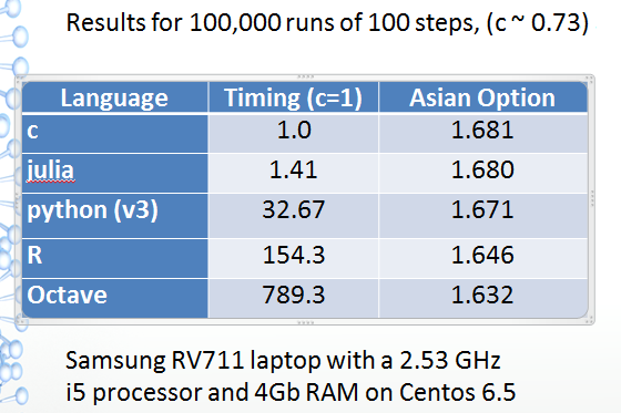
@printf "Option Price: %10.4f\n\n" asianOpt(K = 102.0);

Option Price:     1.6600

runs = 1000000
tm = @elapsed asianOpt(runs, K=102.0)
@printf "Elapsed time for %d runs is %7.4f sec.\n\n" runs tm

Elapsed time for 1000000 runs is  3.5874 sec.

macroexpand(:(@elapsed asianOpt(runs, K=102.0)))

quote  # util.jl, line 68:
    local #1206#t0 = Base.time_ns() # line 69:
    local #1207#val = asianOpt(runs,K=102.0) # line 70:
    Base./(Base.-(Base.time_ns(),#1206#t0),1.0e9)
end

macroexpand(:(@printf "Elapsed time for %d simulations is %7.3f sec.\n\n" runs tm ))

PyJulia adds a Python 'julia' module

Get source from github and use setup.py

Pkg.add("pyjulia")

cd ~/.julia/v0.3/pyjulia
python setup.py install

Speeding up Python execution times

$ python
Python 2.7.9 |Anaconda 2.1.0 (x86_64)
[GCC 4.2.1 (Apple Inc. build 5577)] on darwin

>>> import time as tm
>>> start = tm.time()
>>> asianOpt(1000000,K=102.0)
1.6409
>>> print 'It took', tm.time()-start, 'seconds.'
It took 77.332 seconds.

>>> import julia
>>> jl = julia.Julia()

>>> print jl.bessely0(1.5)
0.3824489237977

>>> import numpy as np
>>> print np.sin(0.5) * jl.bessely0(1.5)
0.1833557812803

>>> jl.require("asian-opt")
>>> jl.asianOpt()
AttributeError: 'Julia' object has no attribute 'asianOpt'

>>> jl.eval("asianOpt(1000000,K=102.0)")
1.6775348594420794

>>> jl.eval("@elapsed asianOpt(1000000,K=102.0)")
3.146388532

$ more myfinx.py

import datetime
import numpy as np
import matplotlib.colors as colors
import matplotlib.finance as finance
import matplotlib.dates as mdates
import matplotlib.ticker as mticker
import matplotlib.mlab as mlab
import matplotlib.pyplot as plt
import matplotlib.font_manager as font_manager

def moving_average(x, n, type='simple'):
    """
    compute an n period moving average.
    type is 'simple' | 'exponential'
    """

def relative_strength(prices, n=14):
    """
    compute the n period relative strength indicator
    http://stockcharts.com/school/doku.php?id=chart_school:glossary_r#relativestrengthindex
    http://www.investopedia.com/terms/r/rsi.asp
    """

def moving_average_convergence(x, nslow=26, nfast=12):
    """
    compute the MACD (Moving Average Convergence/Divergence) using a fast and slow exponential moving avg'
    return value is emaslow, emafast, macd which are len(x) arrays
    """

def run(ticker):
    startdate = datetime.date(2000,1,1)
    today = enddate = datetime.date.today()
    ............
    ............
    ............
    plt.show()

using PyCall

@pyimport myfinx as fx
fx.run("MSFT")

 

• Julia Main Page : http://www.julialang.org
• Julia Wiki Book : https://en.wikibooks.org/wiki/Introducing_Julia
• London Julia UG : http://londonjulia.org

• JuliaStats Group : http://JuliaStats.org
• JuliaOpt Group   : http://JuliaOpt.org
• JuliaQuant Group : https://github.com/JuliaQuant

• JuliaFinMetriX : https://github.com/JuliaFinMetriX
• JuliaEconomics : http://juliaeconomics.com/tutorials
• Quant-Econ.net : http://quant-econ.net

• Steven Johnson EuroSciPy 2014 Keynote Speech : https://www.youtube.com/watch?v=jhlVHoeB05A

• Contact ME : malcolm@amisllp.com